
Considerations for optimizing media retrieval systems using multimodal embeddings
How to build search across video, audio, images and documents using a shared embedding space
Video, audio and image content are pervasive in business data. Search systems that once handled text alone are being asked to retrieve moments from hours-long recordings, match visual scenes to natural language descriptions and surface audio events buried in media libraries. Multimodal embedding models, which map different content types into a shared vector space, are the foundation for making this work.
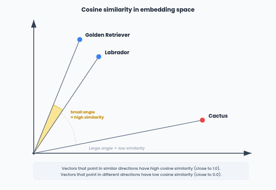
As a refresher, an embedding is a numerical vector that captures the semantic meaning of a piece of content. Two embeddings that are close together in vector space represent content that is similar in meaning, regardless of whether the original inputs were text, images, or audio.
With the release of Google's Gemini Embedding 2 in March 2026, the barrier to building multimodal retrieval systems dropped significantly. For the first time in the Gemini API, a single model maps text, images, video, audio and PDF documents into a unified embedding space, supporting cross-modal search across over 100 languages. But generating embeddings is only half the problem. The harder question is what you do with them once they exist and that is where architectural decisions have real consequences for retrieval quality, operational complexity and long-term flexibility.
This article walks through two architectural approaches for multimodal retrieval (fused embeddings and multi-vector retrieval) and then explores how to handle modality weighting, which is where most production systems either succeed or subtly degrade. We will use Gemini Embedding 2 as the reference model throughout, but the patterns apply broadly to any multimodal embedding model that supports separate per-modality embeddings.
The landscape before Gemini Embedding 2
Before Gemini Embedding 2, building multimodal retrieval meant either using a video-native platform like Twelve Labs Marengo with proprietary pipelines, stitching together multiple single-modality models (CLIP for images, a separate audio encoder, a text embedder), or working with earlier Google offerings like multimodalembedding@001, which handled text, image and video but was limited to 1408 dimensions. Gemini Embedding 2 collapses that into a single API call across five modalities.
Twelve Labs Marengo is the most direct comparison to Gemini Embedding 2 since both offer multimodal embeddings across video, audio, image and text in a unified vector space. When comparing the cost of Twelve Labs Marengo versus Gemini Embedding 2, for video embedding, Gemini Embedding 2 is generally less expensive (roughly $0.00079 per frame vs. Twelve Labs at $0.042 per minute). For audio embedding, the two are close: Gemini charges $0.00016 per second (roughly $0.0096 per minute) compared to Twelve Labs at $0.008 per minute, making Twelve Labs slightly cheaper for audio. For image embedding, pricing is nearly identical at $0.00012 per image (Gemini) vs. $0.0001 per image (Twelve Labs). For text embedding, Gemini charges $0.20 per million tokens while Twelve Labs charges $0.070 per 1K requests, though direct comparison is difficult since the billing units differ.
Note that Twelve Labs also charges a separate infrastructure fee of $0.0015 per minute on top of embedding costs and search queries are billed at $4 per 1K queries, so the total cost of a Twelve Labs pipeline can extend significantly beyond the embedding prices listed earlier in this article.
For teams using a transcription-first approach where text embedding is the primary cost, it is worth noting that OpenAI text-embedding-3-small is priced at $0.02 per million tokens, 10x cheaper than Gemini for text. The trade-off is that OpenAI embeddings are text-only and live in a separate vector space, so you would need to re-embed if you later expand to multimodal retrieval with Gemini. Gemini also offers a free tier for all embedding modalities, though data submitted on the free tier may be used to improve Google products.
Why separate modality embeddings matter
On a high level, rather than being a single signal, a video is a synchronized bundle of what happens visually over time, what is heard (including non-speech sound) and what is said (speech content). Collapsing these into a single undifferentiated vector forces the model to "average" incompatible evidence types. A dialogue query gets diluted by visual data. A sound-event query gets drowned out by scene descriptions.
The key insight with Gemini Embedding 2 is that you control how embeddings are structured through how you call the API. Passing multiple modalities as separate entries in the contents array produces individual embeddings per modality. Bundling them into a single Content object with multiple parts produces one aggregated embedding. This is an API-level design choice that maps directly to the two architectural approaches we will cover.
Because all modalities live in the same geometric space, the query itself does not have to be text. A user can search by uploading an image ("find me other clips that look like this"), by providing an audio snippet ("find moments that sound like this"), or by dropping in a short video clip. The embedding model maps the query into the same space as the indexed content, so similarity comparisons work regardless of whether the query and the result share a modality. Text-to-video, image-to-audio, video-to-video: they all reduce to the same nearest-neighbor lookup. This is what makes a shared multimodal embedding space fundamentally more powerful than running separate, modality-specific search systems side by side.
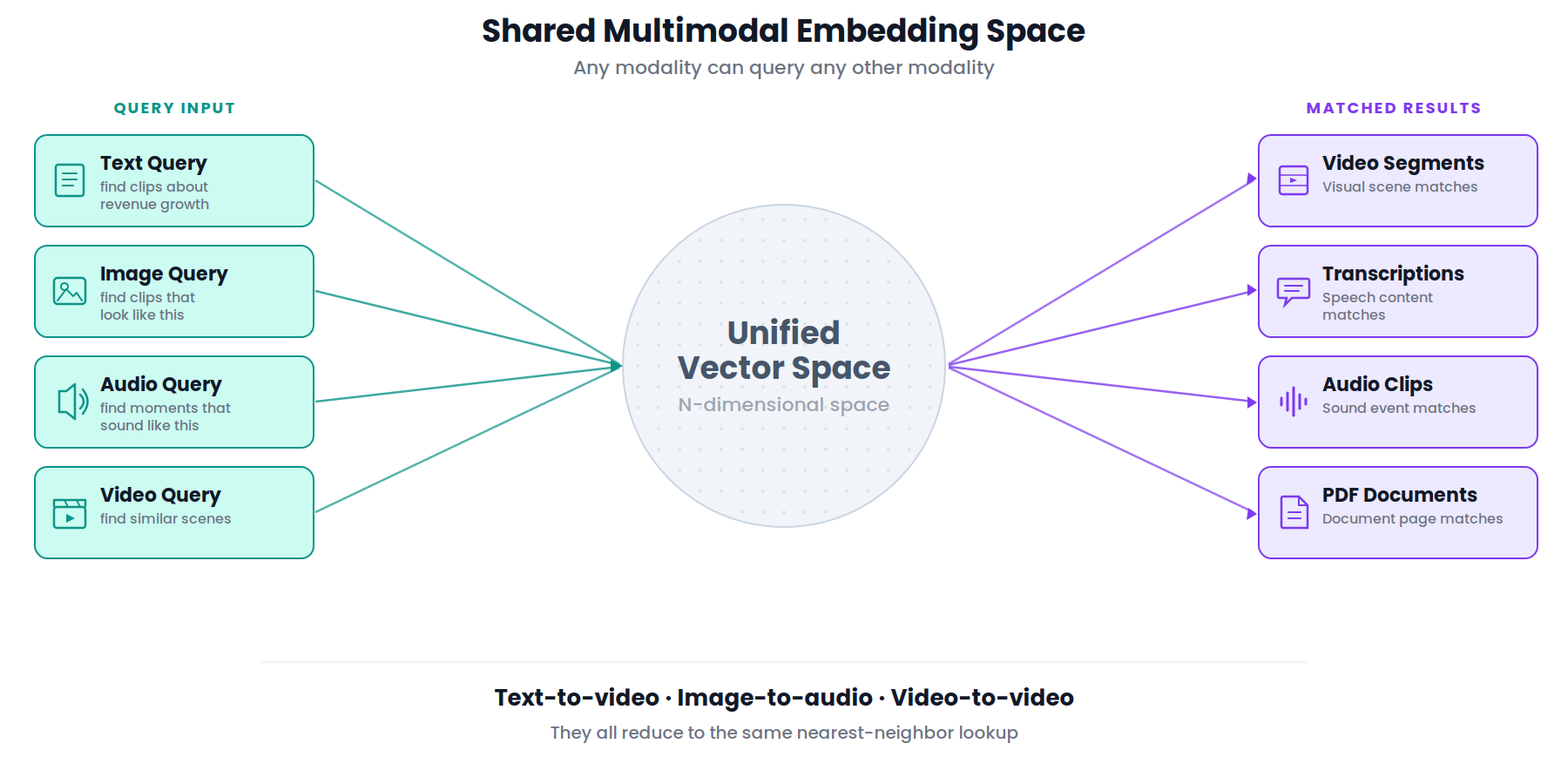
A query like "show me the moment the crowd goes crazy" should primarily hit the audio embedding. "Find the clip where they say 'net revenue retention'" should primarily hit transcription. "Find the play where the defender slides and blocks the shot" should primarily hit visual. The question is: how do you store, query and rank across these separate vectors?
The standard text RAG pipeline
For context, the architecture this article extends is the standard text-based RAG pipeline: embed a query, search a vector database for similar content, retrieve the matching chunks and pass them as context to a generative model. This is a well-understood pattern that most engineering teams have either built or encountered.
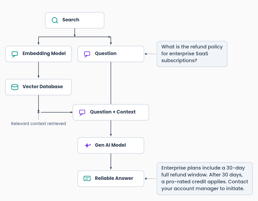
This pipeline works well when your content is text. It breaks down when the information you need to retrieve lives in a video frame, an audio clip, or a spoken sentence that was never written down. That is the problem multimodal embeddings solve.
Everything that follows in this article is about what changes when your content expands beyond just text to video, audio and images and how your embeddings need to capture multiple modalities in the same space
Approach 1: fused embeddings
The simplest path is to combine multiple modality inputs into a single embedding per content segment at ingestion time. With Gemini Embedding 2, you can do this natively by passing all modalities as parts within a single content entry:
from google import genai
from google.genai import types

client = genai.Client()

result = client.models.embed_content(
    model='gemini-embedding-2-preview',
    contents=[
        types.Content(
            parts=[
                types.Part.from_bytes(data=video_frame_bytes, mime_type='image/png'),
                types.Part.from_bytes(data=audio_bytes, mime_type='audio/mpeg'),
                types.Part(text=transcript_text),
            ]
        )
    ]
)

# Single fused embedding
fused_embedding = result.embeddings[0].values
The model returns one embedding that captures information across all provided modalities. You index that single vector in your database and search it exactly like any text-based RAG system: one index, one query, one retrieval pass.
Gemini Embedding 2 outputs 3072-dimensional embeddings by default, but supports flexible dimensionality from 128 to 3072 via the output_dimensionality parameter. The model uses Matryoshka Representation Learning (MRL), which means you can truncate to 768 or 1536 dimensions with minimal quality loss. This is a useful lever for managing storage costs at scale.
Alternatively, if you want more control over the fusion weights, you can generate separate embeddings and fuse them yourself with a weighted sum, then L2-normalize the result:
The L2 normalization step is important. It ensures the fused vector has unit norm, which is required for cosine similarity to work correctly as a distance metric during retrieval. Without normalization, the magnitude of the fused vector would vary depending on the weights and the alignment of the input embeddings, producing inconsistent similarity scores. A typical starting point for visually-heavy content might weight visual at 0.7, audio at 0.15 and transcription at 0.15.
Where fused embeddings work well
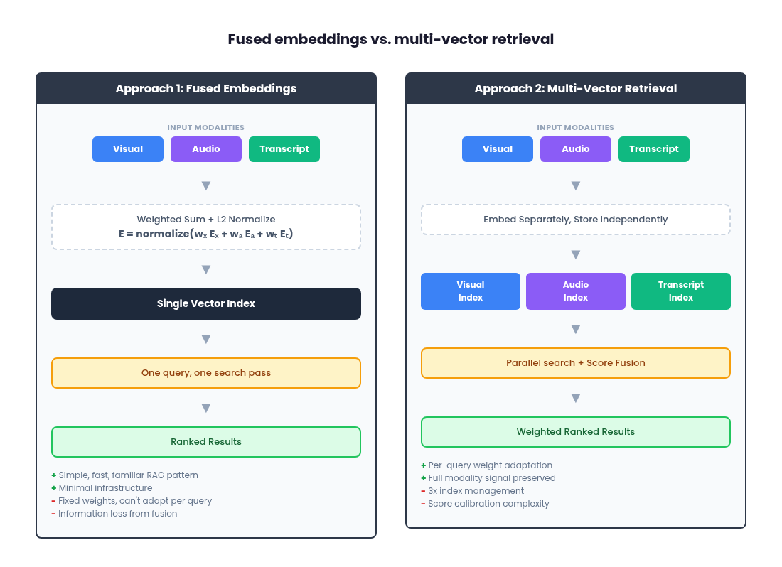
Fused embeddings are the fastest path to a working baseline. You get a single index, a single retrieval pass, no multi-index orchestration and no score-fusion logic at query time. It follows the same patterns as existing text-based RAG architectures, which means your team's existing tooling and mental models transfer directly. For long-form content where segment counts get large, fusion keeps your vector DB footprint and query fan-out minimal.
Where fused embeddings breaks down and why accuracy suffers
Fusion intentionally introduces a bias. You are deciding once, at ingestion time, what the system should "care about." The weights are fixed, whether set by the model's internal aggregation or by your explicit weighted sum. A system tuned for visual-heavy retrieval will systematically underperform for speech-heavy queries or audio-event queries. You can statistically optimize the fixed weights for historical queries, but the system cannot adapt on a per-query basis.
This is a fundamental accuracy trade-off. When you collapse three modality-specific vectors into one, you lose information. The fused vector is a compromise: it cannot fully represent the visual signal, the audio signal and the transcription signal simultaneously. For queries that align with the dominant weight (typically visual), accuracy is comparable to multi-vector retrieval. But for queries that depend on a minority modality, like finding a specific spoken phrase or identifying a sound event, the relevant signal has been diluted by the fusion process and retrieval precision drops. The more diverse your query distribution across modalities, the more accuracy you leave on the table with fusion.
Fusion also obscures failure modes. When retrieval quality drops, you cannot easily isolate whether the issue is the weight choice, modality-specific embedding quality for your domain, segmentation decisions, or the fusion operation itself. And fusion is irreversible. If you later decide to move to a multi-vector architecture, you will need to reprocess your entire content library or maintain duplicate storage of the original separate embeddings.
This architecture is ideal for teams with prior experience building single-vector RAG systems who want the simplest, lowest-risk architecture that still delivers sufficient retrieval quality. Deployments where queries are predominantly single-modality. Early-stage projects where you want a familiar baseline before introducing more moving parts.
Approach 2: multi-vector retrieval
The alternative is to keep all modality embeddings separate and combine them only at search time. With Gemini Embedding 2, you generate separate embeddings by passing each modality as its own entry in the contents array:
from google import genai
from google.genai import types

client = genai.Client()

# Extract modalities from your video segment
visual_frames = [types.Part.from_bytes(data=frame_bytes, mime_type='image/png')]
audio_clip = types.Part.from_bytes(data=audio_bytes, mime_type='audio/mpeg')
transcript = "The quarterly revenue exceeded expectations..."

# Generate separate embeddings in one API call
result = client.models.embed_content(
    model='gemini-embedding-2-preview',
    contents=[
        visual_frames[0],   # Visual embedding
        audio_clip,          # Audio embedding
        transcript,          # Transcription embedding
    ]
)

visual_emb = result.embeddings[0].values
audio_emb = result.embeddings[1].values
transcript_emb = result.embeddings[2].values
You now have three distinct vectors per segment, all living in the same geometric space (which is what makes cross-modal comparison possible), but stored and queried independently.
The pipeline has three stages:
1. Index
For each content segment, persist each modality embedding separately. You can store all modalities in a single vector index with a modality type field for filtering, or use entirely separate indices per modality. Separate indices give you independent scaling (useful if your workload is transcription-heavy, for example) but add operational surface area.
2. Query
At query time, run separate parallel searches against each modality index. There are three querying strategies worth considering. First, direct selection of a single modality, where the user or system chooses which index to search. Second, use the same query embedding across all modalities, using the shared latent space to get results from visual, audio and transcription simultaneously. Third, use an LLM to decompose a complex query into modality-specific sub-queries before searching.
Because Gemini Embedding 2 maps all modalities into a unified space, a single text query embedding can be meaningfully compared against visual, audio and transcription embeddings via cosine similarity. You embed the query once and fan it out across indices.
A practical limitation to be aware of: cross-modal comparisons are inherently noisier than same-modality comparisons. A text query compared against transcription embeddings (text-to-text) will generally produce higher and more reliable similarity scores than the same text query compared against visual embeddings (text-to-image). The unified embedding space makes cross-modal comparison possible, but it does not make it equivalent. Teams should expect lower absolute scores and wider variance from cross-modal indices and plan their per-modality thresholds and fusion weights accordingly. We cover score distributions in more detail in the similarity score thresholds section in this article.
An important caveat on the LLM approach: if you ask the LLM to output modality weights, use structured outputs with constrained schemas (e.g., Pydantic models) rather than free-form numeric generation. Unstructured weight "guesses" are not grounded or reliably calibrated and small changes in prompt wording yield different outputs. We will cover this pattern in detail in the LLM query parsing section.
3. Rank
Merge the parallel result sets into a single ranked list. Two foundational strategies:
Rank-based fusion uses only the rank positions of results across modalities. Reciprocal Rank Fusion (RRF) is a common choice:
This is simple and does not require score calibration, but it discards the actual similarity scores.
Score-based fusion computes a weighted sum of cosine similarities across modalities:
This preserves more signal but introduces a calibration problem. A cosine similarity of 0.85 from the visual index does not "mean the same thing" as 0.85 from the transcription index. Naively combining raw scores can produce unintuitive rankings.
Where multi-vector retrieval works well
Multi-vector retrieval preserves modality-specific signal fidelity. Each embedding retains its full representational power in its own index, avoiding the information loss and averaging artifacts of fusion. You get transparent, modality-level debuggability: when a result is unexpectedly ranked, you can isolate whether the visual match, the transcript similarity, or the audio contributed. And it decouples indexing decisions from ranking decisions. You can adjust modality weights, experiment with fusion strategies, or respond to shifts in query behavior without re-indexing a single piece of content.
Where multi-vector retrieval gets hard and the latency cost.
Three indices means three times the write paths, three times the index management and three times the failure surface. Score calibration across modalities is non-trivial. And you need explicit fusion/ranking logic, which introduces a new design surface that does not exist in single-index systems.
The latency impact deserves specific attention. With fused embeddings, you execute a single vector search against a single index. That is your baseline. With multi-vector retrieval, you are executing three parallel searches plus a ranking/fusion step. Even with parallel execution, your total query latency is bounded by the slowest modality index to return, plus the time to merge and re-rank results. At scale, this fan-out pattern compounds: more shards per index, more network hops, more tail-latency variance. If you add dynamic routing (anchor similarity computation or LLM query parsing), that is additional compute before the search even begins. For latency-sensitive applications, this overhead needs to be carefully benchmarked and budgeted. The accuracy gains from multi-vector retrieval are real, but they come at a measurable latency cost that increases with corpus size and query volume.
This is best for teams that require transparency and debuggability in their retrieval pipeline:
Deployments with mixed query intent across modalities.
Organizations building toward state-of-the-art semantic search where tuning and calibration over time is essential.
Enterprise environments where modality-specific scaling may be required.
What type of content are you querying?
Before diving into model constraints and infrastructure decisions, it is worth stepping back and asking a more fundamental question: what does your content actually look like and how do your users search for it?
The optimal architecture depends heavily on the nature of your media library. A surveillance camera feed is almost entirely visual, with no meaningful audio or speech. A podcast library is dominated by spoken dialogue, with no visual signal at all. A training video library might have all three modalities in roughly equal proportion. Social media content, particularly short-form video on platforms like TikTok or Instagram Reels, is often dominated by narration or voiceover laid over visual content, meaning the transcription embedding may carry more retrieval value than the visual embedding for most queries, even though the content is technically "video."
This matters because the right weighting strategy and even the right architectural approach, varies with your content profile. If you are building search for a library of conference talks, the transcription index will handle the majority of useful queries ("find where the speaker discusses pricing strategy") and investing heavily in visual embeddings may not improve retrieval quality much. Conversely, if you are building search for a sports highlight library, visual embeddings are primary and transcription is secondary at best.
Think about this in terms of signal density per modality. For each content type in your library, ask: where does the retrievable information actually live? If 80% of your queries will be answered by one modality, a fused embedding approach with weights skewed toward that modality might be perfectly sufficient. If your queries genuinely span modalities ("find the moment the coach reacts on the sideline while the announcer says 'unbelievable'"), multi-vector retrieval becomes essential.
The content profile also affects your chunking strategy, your score thresholds and your evaluation dataset design. Understanding your content before choosing your architecture will save you from over-engineering for modalities that do not matter or under-investing in the ones that do.
Transcription-first as a legitimate version 1
For a large class of real-world video content (talking heads, interviews, podcasts, conference talks, webinars, social media narration), transcription embeddings alone will get you 80 to 90 percent of your retrieval quality at a fraction of the infrastructure cost. This is a pragmatic starting point and compromise that many teams should seriously consider before building a full multimodal pipeline.
The reasoning is straightforward. If the retrievable information in your content lives primarily in what people say, then a text embedding of the transcript captures the signal your users are actually searching for. You run speech-to-text on your media library, chunk the transcripts, embed them with Gemini Embedding 2 as plain text and index those embeddings in a single vector store. Your query pipeline is identical to a standard text RAG system. No multi-index orchestration, no score fusion, no modality weighting. One index, one query, one retrieval pass.
You also get a major UX advantage for free: timestamps. Speech-to-text output includes word-level or segment-level timestamps, which means your search results can link directly to the exact moment in a video where the relevant content occurs. Instead of surfacing a 45-minute conference talk and asking the user to scrub through it, you surface a link that jumps to minute 23:14 where the speaker discusses pricing strategy. This is a significantly better user experience than what you get from embedding video frames, where temporal granularity depends entirely on your chunking strategy and you lose the ability to pinpoint exact moments.
The cost difference is also substantial (more on this in the cost section). Embedding a transcript as text is orders of magnitude cheaper than embedding the equivalent duration of raw video or audio. For teams evaluating whether to go multimodal, the honest question is: does your content and your query distribution actually require visual or audio embeddings, or are you adding complexity for modalities that will not meaningfully improve retrieval quality?
Start with transcription. Measure retrieval quality against real user queries. If you find consistent failure cases where the transcript does not capture the relevant signal ("find the moment the product demo crashes on screen," "find clips with applause"), that is your evidence for adding visual or audio modalities. Without that evidence, a full multimodal pipeline is over-engineering.
One thing to get right from day one: design your schema and metadata so that adding visual or audio embeddings later does not require restructuring your database. Each indexed transcript chunk should store the source content ID, the start and end timestamps and any relevant metadata (speaker, content type, date). When you later add a visual embedding index, you create entries with the same content IDs and timestamp ranges, making it trivial to correlate results across modality indices. If your transcription-only system stores segment identifiers and temporal metadata cleanly, the migration to multi-vector retrieval is additive. You are adding new indices alongside the existing one rather than rebuilding from scratch.
Embedding each modality: what you are actually producing
It is worth being explicit about what a multimodal embedding model gives you and how the pieces fit together, because the terminology can be misleading.
With Gemini Embedding 2, you can embed five types of input: text, images, video, audio and PDF documents. Each of these produces a vector in the same shared embedding space. That shared space is what makes cross-modal retrieval possible. A text query and a video frame both become vectors in the same 3072-dimensional space and cosine similarity between them is meaningful.
For a video retrieval system, you typically do not embed the raw video file as a single unit. Instead, you decompose it into its constituent signals and embed each one separately:
Visual frames or clips
Extract key frames or short clips and embed them as images or video segments. These capture what is on screen: scenes, objects, people, actions and on-screen text. The model can distinguish text in images similar to OCR, so text overlays, titles and captions in video frames are captured in the visual embedding. If you need to search specifically for on-screen text rather than visual content, consider prepending your query with a clarifier like 'the text' to disambiguate (e.g., 'the text pricing' vs. 'a slide about pricing').
Audio track
Extract the audio and embed it separately. This captures non-speech sounds like music, ambient noise, applause, sirens, or tone. Note that Gemini Embedding 2 does not process audio tracks within video files, so this extraction step is mandatory. By default, audio tracks are not processed when you embed a video file. Google’s Vertex AI documentation indicates that audio extraction can be enabled as an option, which reduces the maximum video duration from 120 seconds to 80 seconds. Regardless of whether you enable audio extraction, the result is still a single fused embedding. If your architecture requires separate audio embeddings for independent weighting or querying, you still need to extract and embed audio as a standalone input.
Transcription
Run speech-to-text on the audio to produce a transcript, then embed the text. This captures the semantic content of what is being said: dialogue, narration, voiceover.
A critical implementation detail that is easy to miss: Gemini Embedding 2 does not process the audio track when you embed a video file. It only processes the visual frames. This means that embedding a video does not give you audio or speech coverage. If you hand the model a video of a keynote speech and embed it as-is, the resulting vector captures what the stage looks like, not what the speaker is saying. You are always doing separate extraction work for audio and transcription, regardless of which architectural approach you choose. Many teams assume that "multimodal video embedding" captures everything in the file. It does not and building your pipeline on that assumption will produce a system that fails on speech-heavy queries.
Each of these becomes its own embedding vector. You can then choose to combine them into a single fused vector (Approach 1) or store them in separate indices (approach 2). Either way, the raw material is the same: distinct vectors per modality, all comparable in the same geometric space.
You can also embed other content types alongside video. PDF documents, product images, standalone audio files and plain text can all be embedded with the same model and stored in the same indices. This means your retrieval system is not limited to video. A query could match a video segment, a PDF page and a product photo, all ranked together in a single result set.
Video search vs. search within video
There is a critical distinction that teams often miss until late in development: "video search" (which video matches my query?) is a fundamentally different product experience from "search within video" (where in this video does the relevant moment occur?). Users almost always want the latter. When someone searches for "the moment the speaker discusses pricing strategy," they do not want a link to a 45-minute keynote. They want to land at minute 23:14.
Gemini Embedding 2 produces one embedding per video input. If you embed a 2-minute clip, you get a single vector with no temporal metadata attached. You know this video matched, but you do not know where in the video. Building search-within-video requires you to construct the segmentation and timestamp pipeline yourself before calling the embedding API.
The segment-level pipeline
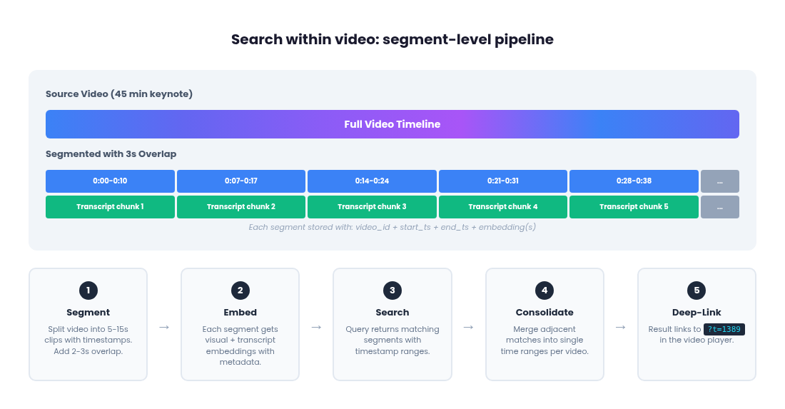
The full pipeline for timestamp-precision video search has five steps:
1. Segment the video with timestamp metadata
Before embedding anything, split your source video into short segments (5 to 15 seconds each) and track the start and end timestamps for each segment. This is the step Gemini does not do for you and it is where most of the implementation work lives.
You have two options. Fixed-length segmentation (every N seconds) is simple and predictable but can split scenes awkwardly. Dynamic scene-based segmentation using tools like PySceneDetect detects visual transitions and produces semantically coherent segments at the cost of variable lengths.
For timestamp-precision search, overlapping segments are near-essential, not optional. If a key moment falls exactly on a chunk boundary, both adjacent segments will have a degraded representation of it. Adding a 2 to 3 second overlap between segments is cheap insurance: it slightly increases your embedding count but dramatically reduces the chance of a relevant moment being poorly represented because it was split across two chunks.
2. Embed each segment independently
Pass each short clip to Gemini Embedding 2 as a separate video input. Each call returns a single embedding for that segment. Store the embedding alongside the segment's source video ID, start timestamp and end timestamp as metadata in your vector database.
3. Align audio and transcription to the same timestamp ranges
For each visual segment, extract the corresponding audio slice and transcription chunk covering the same time range. Embed each separately. You now have up to three embeddings per segment (visual, audio, transcription), all sharing the same content ID and timestamp range.
The transcription track has a natural advantage here: speech-to-text gives you word-level timestamps for free, so you can chunk transcripts precisely by sentence or topic boundary and still know the exact timestamp. Visual segments do not have that precision. You are imposing boundaries from outside.
4. At query time, return timestamps, not just video IDs
When a search matches a segment embedding, the result includes the source video ID and the start/end timestamps from the metadata. The UI deep-links directly to that moment in the video player.
5. Consolidate adjacent matching segments
A single concept often spans multiple consecutive segments. If segments 3, 4 and 5 of a video all score highly for a query, the UI should merge them into one result spanning the full time range rather than showing three separate results from the same video. This is a post-retrieval step: group results by source video ID, merge contiguous or overlapping timestamp ranges and present the merged range as a single result.
Full video segmentation pipeline example
Here is the complete loop from source video to timestamped search results:
import subprocess
import json
import os
from google import genai
from google.genai import types

client = genai.Client()

# --- Step 1: Segment the video ---

def segment_video(video_path, segment_duration=10, overlap=3):
    """Split a video into overlapping segments with timestamps."""
    # Get video duration using ffprobe
    probe = subprocess.run(
        ['ffprobe', '-v', 'quiet', '-print_format', 'json', '-show_format', video_path],
        capture_output=True, text=True
    )
    duration = float(json.loads(probe.stdout)['format']['duration'])

    segments = []
    start = 0.0
    step = segment_duration - overlap

    while start < duration:
        end = min(start + segment_duration, duration)
        output_path = f"/tmp/segment_{start:.1f}_{end:.1f}.mp4"
        subprocess.run([
            'ffmpeg', '-y', '-i', video_path,
            '-ss', str(start), '-to', str(end),
            '-c:v', 'libx264', '-an', output_path
        ], capture_output=True)
        segments.append({
            'path': output_path,
            'start': start,
            'end': end,
        })
        start += step

    return segments

# --- Step 2 & 3: Embed each segment with all modalities ---

def embed_segment(segment, video_id, transcript_chunks):
    """Embed visual, audio and transcription for one segment."""
    # Visual embedding
    with open(segment['path'], 'rb') as f:
        video_bytes = f.read()

    visual_result = client.models.embed_content(
        model='gemini-embedding-2-preview',
        contents=[types.Content(parts=[
            types.Part.from_bytes(data=video_bytes, mime_type='video/mp4')
        ])],
    )

    # Find transcript chunks overlapping this segment's time range
    matching_text = ' '.join([
        chunk['text'] for chunk in transcript_chunks
        if chunk['start'] < segment['end'] and chunk['end'] > segment['start']
    ])

    # Prepend document instruction for indexing
    doc_text = f"title: none | text: {matching_text}" if matching_text else '[no speech]'
    text_result = client.models.embed_content(
        model='gemini-embedding-2-preview',
        contents=[doc_text],
    )

    return {
        'video_id': video_id,
        'start': segment['start'],
        'end': segment['end'],
        'visual_embedding': visual_result.embeddings[0].values,
        'transcript_embedding': text_result.embeddings[0].values,
        'transcript_text': matching_text,
    }

# --- Step 4: Query with timestamp results ---

def search_segments(query, index, top_k=20, threshold=0.25):
    """Search and return timestamped results."""
    # Prepend retrieval instruction for query embedding
    query_with_instruction = f"task: search result | query: {query}"
    query_result = client.models.embed_content(
        model='gemini-embedding-2-preview',
        contents=[query_with_instruction],
    )
    query_emb = query_result.embeddings[0].values

    # Search your vector index (pseudocode - depends on your DB)
    raw_results = index.search(query_emb, top_k=top_k)

    return [
        r for r in raw_results
        if r['score'] >= threshold
    ]

# --- Step 5: Consolidate adjacent segments ---

def consolidate_results(results, max_gap=3.0):
    """Merge consecutive segments from the same video into single results."""
    from itertools import groupby

    # Group by video ID
    results.sort(key=lambda r: (r['video_id'], r['start']))
    consolidated = []

    for video_id, group in groupby(results, key=lambda r: r['video_id']):
        segments = list(group)
        current = {
            'video_id': video_id,
            'start': segments[0]['start'],
            'end': segments[0]['end'],
            'best_score': segments[0]['score'],
        }

        for seg in segments[1:]:
            # If this segment is contiguous or overlapping, merge it
            if seg['start'] <= current['end'] + max_gap:
                current['end'] = max(current['end'], seg['end'])
                current['best_score'] = max(current['best_score'], seg['score'])
            else:
                consolidated.append(current)
                current = {
                    'video_id': video_id,
                    'start': seg['start'],
                    'end': seg['end'],
                    'best_score': seg['score'],
                }
        consolidated.append(current)

    consolidated.sort(key=lambda r: r['best_score'], reverse=True)
    return consolidated

# --- Putting it together ---

video_path = 'keynote_recording.mp4'
video_id = 'keynote-2026-03'

# Assume transcript_chunks comes from your speech-to-text pipeline,
# each with 'text', 'start', 'end' fields
transcript_chunks = run_speech_to_text(video_path)  # your STT function

segments = segment_video(video_path, segment_duration=10, overlap=3)
records = [embed_segment(seg, video_id, transcript_chunks) for seg in segments]

# Insert records into your vector database with metadata...
# Then at query time:
# results = search_segments("discusses pricing strategy", index)
# final = consolidate_results(results)
# -> [{'video_id': 'keynote-2026-03', 'start': 1389.0, 'end': 1412.0, ...}]
# -> Deep-link: keynote_recording.mp4?t=1389
The cost of segment-level precision
This pipeline produces significantly more embeddings than a single-vector-per-video approach. A 10-minute video chunked into 10-second segments with 3-second overlap generates roughly 86 visual embedding calls. Add transcription embeddings for each segment and you are approaching 170 calls for one video. Multiply that across a library of thousands of hours and the embedding cost grows quickly.
This is another reason the transcription-first approach is compelling for search-within-video. With transcription, you do not need to segment video files at all. Speech-to-text gives you timestamped text, you chunk it by sentence or paragraph boundaries and each text embedding call is a fraction of the cost of a video embedding call. You get timestamp-precision search results with dramatically less implementation work and cost. The visual segmentation pipeline described earlier is only necessary when you need to search by what is shown in the video, not by what is said.
For teams that do need visual search, consider a tiered approach: embed transcription for your entire library (cheap, fast, gives you timestamp-level search for speech content), then selectively add visual embeddings for content categories where transcription alone fails to capture the relevant signal. This avoids paying the full visual segmentation cost for content where it does not improve retrieval quality.
Practical considerations with Gemini Embedding 2: video chunking strategies
Gemini Embedding 2 supports video up to 120 seconds, processing a maximum of 32 frames (1 fps for short videos, uniformly sampled for longer ones). Audio tracks within video files are not processed, so you need to extract and embed audio separately. For content longer than 120 seconds, you will need to chunk videos into overlapping segments and embed each chunk individually.
The chunking strategy you choose has a direct impact on retrieval quality and index size. There are a few common approaches:
Fixed-length chunking
Splits the video into segments of uniform duration, for example 30 or 60 seconds. This is simple to implement and produces predictable index sizes, but it can split a coherent scene across two chunks, reducing the quality of both embeddings. It works best when your content does not have strong narrative structure, like surveillance footage or continuous event recordings.
Scene-based chunking
Detects visual shot boundaries or significant transitions and splits the video at those points. This produces more semantically coherent segments, since each chunk corresponds to a distinct visual scene. The trade-off is variable segment lengths, which can complicate batching and storage planning. Scene detection can be done with open-source tools like PySceneDetect.
Overlapping chunks
Add a buffer (typically 2 to 5 seconds) between adjacent segments. If you are building search-within-video (see the pipeline section earlier in this article), overlapping segments should be treated as near-essential rather than optional. Without overlap, key moments that fall on a chunk boundary are poorly represented in both adjacent segments and your search will miss them. The cost of overlap is a modest increase in embedding count. The cost of not overlapping is missed results at the exact moments users are searching for.
For the audio and transcription tracks, your chunking strategy should align with the visual segmentation but does not have to be identical. Audio can be chunked by silence detection or fixed intervals and transcription can be chunked by sentence or paragraph boundaries from the speech-to-text output. The important thing is to maintain a mapping between each embedding (visual, audio, transcription) and its source timestamp range, so that results from different modality indices can be correlated back to the same moment in the video.
Embedding dimensionality & accuracy
The default 3072-dimension embedding output is the highest fidelity option and higher dimensionality generally means higher retrieval accuracy. More dimensions give the model more room to encode fine-grained distinctions between semantically similar content. The difference between "a person running on a track" and "a person jogging through a park" may be captured in dimensions that get discarded at lower sizes. Gemini Embedding 2 uses Matryoshka Representation Learning (MRL), a technique that “nests” information by dynamically scaling down dimensions, which means you can truncate to 768 or 1536 dimensions with graceful quality degradation rather than a cliff, but the accuracy loss is not zero.
Google's published benchmarks for gemini-embedding-001 show MTEB scores dropping from 68.17 at 1536 dimensions to 63.31 at 128, a meaningful difference for precision-sensitive applications. Gemini Embedding 2 scores 69.9 on the MTEB Multilingual benchmark at full dimensionality and supports the same MRL truncation, so expect a similar degradation curve at smaller sizes.
This creates a three-way trade-off between accuracy, storage cost and query latency. Higher dimensions produce better retrieval but require more storage and slower nearest-neighbor search. If you are running multi-vector retrieval with three indices, the dimensionality decision is amplified 3x: cutting from 3072 to 768 dimensions reduces your total vector storage by 75%, but you are also reducing the representational capacity of each modality index. For large libraries, the right dimensionality depends on whether your bottleneck is retrieval quality or infrastructure cost.
Vector normalization, cosine similarity and dot product
This is a detail that is easy to overlook but has real performance implications in production.
Cosine similarity measures the angle between two vectors, ignoring their magnitude. It is the standard distance metric for semantic search because it focuses on directional similarity, which corresponds to conceptual closeness. Values range from -1 (opposite) to 1 (most similar). The formula divides the dot product of two vectors by the product of their magnitudes.
Dot product, on the other hand, is simply the sum of element-wise products. It is computationally cheaper because it skips the magnitude normalization step. Critically, if both vectors are already normalized, cosine similarity and dot product produce identical results. When both vectors have magnitude 1, dividing by the product of their magnitudes is dividing by 1, so cosine similarity reduces to a plain dot product.
This matters for Gemini Embedding 2 specifically. The 3072-dimension embeddings come pre-normalized from the API. If you are using full-dimension embeddings, you can use dot product as your distance metric and get the same ranking as cosine similarity, but with faster computation. At scale, across millions of vectors and thousands of queries per second, that savings adds up.
However, if you truncate to a smaller dimension (768 or 1536), the truncated vectors are no longer normalized. You need to re-normalize them before indexing, or you need to use cosine similarity (which normalizes on the fly) instead of dot product. Failing to do this will produce incorrect rankings, because vectors with different magnitudes will be compared unfairly.
For context, most text-only embedding providers (like those from major cloud providers) also return pre-normalized embeddings, so dot product works out of the box for those too. But those models are text-only and do not support the multimodal use cases we are discussing here. The normalization behavior is a property of the specific model and dimensionality you are using, so always verify it rather than assuming.
In your vector database configuration, this translates to choosing your distance metric. If you know your embeddings are normalized, choose dot product for speed. If there is any chance they are not (truncated dimensions, mixed models, manual fusion), use cosine similarity to be safe.
One practical note about managed vector databases
Many managed vector database services (including S3 Vectors and some configurations of Pinecone and Qdrant) default to or only support cosine similarity as the distance metric and do not expose dot product as an option. If you are using a managed service, check whether you can actually select your distance metric before optimizing for dot product. As mentioned, cosine similarity produces identical rankings to dot product for normalized vectors and the only difference is computational cost. If your managed service hardcodes cosine, that is fine. The ranking quality is the same. The dot product optimization matters most for self-hosted deployments at very high query volumes where you control the index configuration
Task instructions instead of task types
Prior Gemini embedding models used a task_type parameter (e.g., RETRIEVAL_QUERY, RETRIEVAL_DOCUMENT) to tell the model how the embedding would be used. Gemini Embedding 2 does not support this parameter. Instead, you include the task as a natural language instruction directly in your prompt.
In our experience, this means prepending a structured instruction prefix to the text you are embedding. The format follows a key: value | key: value pattern. When indexing content for search, format it as title: {title} | text: {content} (use title: none if there is no title). When embedding a search query, format it as task: search result | query: {content}. The model uses the instruction prefix to adjust its internal representation, similar to how task_type worked in earlier models but with more flexibility since different tasks use different prefix structures.
Google provides specific prefix formats for different use cases: task: search result for search, task: question answering for Q&A, task: fact checking for verification, task: code retrieval for code search, task: classification for classification and task: clustering for clustering. For symmetric tasks like classification or clustering, the format is simpler: task: classification | query: {content}.
This is a meaningful change if you are coming from Gemini Embedding 001 or other models that used explicit task type enums. Your embedding calls no longer pass a task_type config. Instead, you prepend the structured instruction to the content string itself. For retrieval pipelines where both the query and indexed content are text, the asymmetric format (one structure for documents, a different one for queries) helps the model handle the length and specificity mismatch between a terse search query and a multi-sentence transcript chunk.
For non-text modalities (image, video, audio), the instruction-based approach is less impactful since those modalities do not have the same query-vs-document length asymmetry. When a user searches by uploading an image or audio clip rather than typing text, the instruction matters less because there is no length mismatch to compensate for.
Note that as of this writing, the Gemini API documentation (ai.google.dev) does not document the instruction-based format for gemini-embedding-2-preview. The format described earlier comes from the Vertex AI documentation (cloud.google.com), which explicitly states that the task_type parameter is not supported for this model. If you are following the Gemini API docs, be aware that passing task_type in EmbedContentConfig will be ignored for gemini-embedding-2-preview.
Embedding aggregation behavior
The API's behavior around single vs. multiple content entries is the mechanism that enables both architectural approaches. This is worth testing carefully with your specific data, since the model's internal aggregation when fusing modalities within a single content entry may weight modalities differently than you would choose with explicit fusion.
Similarity score thresholds
Not every result your vector search returns is actually relevant. Cosine similarity scores from embedding models follow a distribution where most content clusters in the 0.2 to 0.5 range and truly relevant matches tend to score significantly higher. Returning results with scores under 0.25 almost always introduces noise: content that is technically the "nearest neighbor" but has no meaningful semantic relationship to the query. In practice, applying a minimum similarity threshold of around 0.25 (and often higher, depending on your domain) filters out these low-confidence results before they ever reach the user or the ranking layer.
This is especially important in multi-vector retrieval, where low-scoring results from one modality index can pollute the merged ranking even if the other modalities returned strong matches. The threshold should be tuned per modality, because score distributions differ meaningfully across visual, audio and transcription indices.
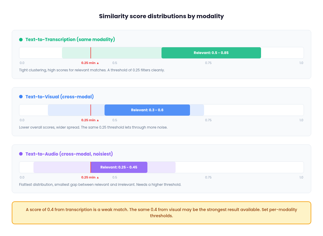
In practice, text-to-text comparisons (query embedding vs. transcription embedding) tend to produce the highest and most tightly clustered similarity scores for relevant matches, often in the 0.5 to 0.8+ range, because both sides are the same modality and the semantic signal is dense. Text-to-visual comparisons (text query vs. image/video embedding) produce lower scores overall, with relevant matches often landing in the 0.3 to 0.6 range, because the cross-modal mapping introduces noise even in a unified embedding space. Text-to-audio comparisons tend to be the noisiest, with flatter score distributions and smaller gaps between relevant and irrelevant results, particularly for non-speech audio like ambient sounds or music.
What this means in practice: a score of 0.4 from your transcription index might be a weak match, while 0.4 from your visual index could be among the strongest results available. If you apply the same threshold across all modalities, you will either over-filter your visual and audio results or under-filter your transcription results. Set per-modality thresholds based on observed score distributions during development and revisit them as your content library grows.
Cost: text vs. video vs. audio embedding
The cost difference between embedding modalities is large enough to influence architectural decisions. With Gemini Embedding 2, text embedding is priced per token, while video and audio embedding is priced per second of media. In practice, embedding a transcript as text is orders of magnitude cheaper than embedding the equivalent duration as raw video or audio.
There is also a frame rate cost dynamic to be aware of. Gemini Embedding 2 processes a maximum of 32 frames per video input. For short videos (32 seconds or less), this means 1 frame per second. For longer videos, the 32 frames are uniformly sampled across the full duration, meaning a 2-minute video is sampled at roughly one frame every 3.75 seconds.
If your content has fast visual changes and you need dense frame coverage, you will want to segment videos into shorter clips (30 seconds or less) to maintain 1 fps sampling. This improves visual embedding quality but multiplies the number of embedding calls.
A 2-minute video embedded as a single call costs 32 frames. The same video segmented into four 30-second clips costs 120 frames, roughly 4x more, but captures 4x more visual detail. The chunking decision extends beyond just retrieval granularity and timestamp precision to also directly affect how much visual information the model sees per second of content
Consider a 10-minute video. Embedding the full video (chunked into segments) requires processing 600 seconds of visual frames. Embedding the extracted audio requires processing 600 seconds of audio. But embedding the transcript of that same 10 minutes might only be a few hundred tokens of text, depending on how much is said. The text embedding call is a tiny fraction of the cost of either media embedding call.
This cost gap compounds quickly at scale. A media library with 10,000 hours of content will cost dramatically more to index with full multimodal embeddings (visual + audio + transcription) than with transcription embeddings alone. And that is just the embedding cost. You also pay more for vector storage (three indices instead of one) and query compute (three searches instead of one) in the multi-vector architecture.
For teams evaluating whether to go beyond transcription, the ROI question is concrete: does adding visual or audio embeddings improve retrieval quality enough to justify the cost increase? If your content is primarily speech-driven and your queries target what people say, the answer is often no. If your content has significant non-speech signal (visual demos, ambient audio, on-screen text not captured by transcription), then the cost is justified. Run the numbers for your specific corpus size and query volume before committing to a full multimodal pipeline.
Model versioning and re-embedding risk
Gemini Embedding 2 is currently in preview (gemini-embedding-2-preview) and its embedding space is not compatible with the previous Gemini Embedding 001. Vectors generated by different model versions cannot be meaningfully compared, which means that if Google changes the model at general availability or releases a successor, you may need to re-embed your entire corpus.
For a small content library, this is an inconvenience. For a large one (tens of thousands of hours of video with visual, audio and transcription embeddings across multiple indices), re-embedding is a significant operational cost in both compute and time. Teams should factor this into their planning. Building on a preview model is reasonable for development and early production, but budget for a potential full re-index when the model stabilizes. This is another argument for the transcription-first approach: if you need to re-embed, re-embedding text transcripts is fast and cheap compared to re-embedding raw video and audio.
Vector index configuration
The embedding model gets most of the attention, but the vector index you store embeddings in has its own set of decisions that affect retrieval quality, latency and cost.
Single index vs. separate indices
For multi-vector retrieval, you have two options: store all modality embeddings in a single index with a metadata field (e.g., modality_type: "visual") and filter at query time, or maintain entirely separate indices per modality. A single index is simpler operationally but means every query touches the full dataset and relies on metadata filtering to scope results. Separate indices let you scale each modality independently (useful if transcription queries dominate your traffic) and let you tune index parameters per modality, but you now have three deployments to manage, monitor and keep in sync. For most teams starting out, a single index with metadata filtering is the pragmatic choice. Move to separate indices when you have concrete evidence that a modality needs independent scaling or tuning.
Approximate nearest neighbor (ANN) algorithms
Most vector databases use ANN algorithms rather than exact search because exact search does not scale. The two most common are HNSW (Hierarchical Navigable Small World) and IVF (Inverted File Index). HNSW gives better recall at query time but uses more memory, because it builds a graph structure that lives in RAM. IVF uses less memory by partitioning vectors into clusters, but requires tuning the number of clusters and the number of probes at query time to balance recall against speed. For most multimodal retrieval workloads where your corpus is under a few million vectors, HNSW with default parameters is the right starting point. You can always tune later.
Metadata schema design
Every vector you store should carry metadata that your pipeline can filter on: video_id, start_ts, end_ts, modality_type and any content-level tags (speaker, topic, content source). Design your metadata schema to support the hard filters your LLM parser will extract. If your parser outputs a filter like {field: "speaker", operator: "equals", value: "CEO"}, that field needs to exist in your index metadata. Think about which filters you will need before you start ingesting, because retrofitting metadata onto millions of existing vectors is painful.
Hybrid search for transcription
For the transcription modality specifically, pure vector search can miss exact keyword matches that a user expects. A query like "find where she says net revenue retention" should surface segments containing that exact phrase, even if the embedding similarity is not the highest scored result. Most production vector databases now support hybrid search, which combines vector similarity with keyword matching (BM25 or equivalent) in a single query. For transcription indices, enabling hybrid search is almost always worth it. It catches the literal matches that embeddings sometimes miss while still benefiting from the semantic understanding that vector search provides. For visual and audio indices, hybrid search is not applicable since there is no text to keyword-match against.
Choosing a vector database
The landscape here is wide, but a few options cover the majority of production use cases.
Qdrant
An open-source tool which can be self-hosted or used as a managed cloud service. It supports HNSW indexing, rich metadata filtering and has strong performance characteristics for multi-vector workloads. It is a good fit for teams that want operational control without building everything from scratch.
Pinecone
A fully managed service and requires zero infrastructure work. You get a hosted index with metadata filtering, hybrid search and namespace-based partitioning out of the box. The tradeoff is cost at scale and vendor lock-in, but for teams that want to focus on retrieval logic rather than database operations, it is the fastest path to production.
pgvector
Extends Postgres with vector similarity search. If your team already runs Postgres, pgvector lets you keep embeddings alongside your relational data without introducing a new database into your stack. It is the simplest option architecturally, though it does not match the query performance of purpose-built vector databases at high scale.
Amazon S3 Vectors
This is a newer option worth evaluating that was launched in 2025. S3 Vectors provides purpose-built vector storage within the S3 ecosystem, with sub-second query latency and no infrastructure provisioning. The pricing model is pay-per-use with no idle capacity costs, which can translate to significant savings (AWS cites up to 90% cost reduction compared to provisioned vector databases) for workloads with variable or infrequent query patterns. It supports metadata filtering, strong write consistency and integrates with Amazon Bedrock and OpenSearch. The tradeoff is that S3 Vectors is optimized for cost and durability rather than ultra-low latency. Query times are sub-second for infrequent queries and around 100ms for sustained traffic, which is fine for most search UIs but may not meet requirements for real-time streaming applications. If you are already in the AWS ecosystem and your query volume is bursty rather than constant, S3 Vectors is worth benchmarking against provisioned alternatives.
The right choice depends on your existing infrastructure, team expertise, query volume patterns and how much operational overhead you are willing to absorb. For a version 1, pick whatever lets you ship fastest. You can migrate later if the indexing layer becomes a bottleneck and if you followed the metadata schema guidance described in this article, your data model will transfer cleanly across databases.
The weight problem: fixed vs. dynamic
Once you have committed to multi-vector retrieval, the central question becomes: how do you determine the modality weights for each query?
Fixed weights with statistical optimization
The most accessible approach is to treat weight selection as an empirical tuning problem. Assemble an evaluation dataset of representative queries with ground truth relevance labels, define a retrieval quality metric (precision@1, recall@K, mAP) and systematically evaluate different weight combinations. In practice, the weight space for three modalities is small enough that you can sweep through combinations at reasonable granularity (e.g., increments of 0.05 or 0.1) and pick the combination that maximizes your metric on a held-out set.
The quality of this process depends entirely on the evaluation dataset. A good eval set for multimodal retrieval should include queries that span all modalities (visual-dominant, speech-dominant, audio-dominant and mixed), include edge cases like negation and hard filters and reflect the actual distribution of queries your users make. If 70% of real queries target transcription but your eval set is evenly split across modalities, you will optimize for a weight balance that does not match production. Sample from real user queries wherever possible, supplement with synthetic queries for underrepresented modalities and ensure you have at least a few dozen queries per modality category to get stable metric estimates.
This produces a single optimal weight set for your corpus. Deploy it as your production configuration and periodically re-evaluate as your content library and query patterns evolve.
The advantage is simplicity. Evaluation metrics, grid sweeps and cross-validation are familiar concepts for any engineering team. It avoids fusion artifacts, preserves debuggability and serves as a natural stepping stone to dynamic routing later.
The limitation is that the weights are still fixed. A transcription-heavy query like "what did she say about Q4 pipeline" gets the same visual-skewed weights as a purely visual query. If your query distribution is homogeneous, this works. If it is diverse, no single weight combination will satisfy all cases.
Intent-based dynamic routing (anchor-based)
You could train a small supervised model to predict per-query weights, but for most teams this is overkill given how reliably out-of-the-box LLMs handle query decomposition (more on that later in this article). A lighter alternative is to construct a small set of "routing anchors": short text descriptions that represent the semantic intent of each modality.
For example:
Visual anchor: "This document contains content about the visual elements of the video."
Audio anchor: "This document contains content about the audio elements of the video."
Transcription anchor: "This document contains content about the spoken words in the audio elements of the video."
Embed the anchors and the incoming query using Gemini Embedding 2. Compute cosine similarity between the query embedding and each anchor embedding, then apply a softmax with a temperature parameter to convert the similarities into normalized weights:
import numpy as np
from google import genai

client = genai.Client()

# Pre-compute anchor embeddings (do this once)
anchors = [
    "This document contains content about the visual elements of the video.",
    "This document contains content about the audio elements of the video.",
    "This document contains content about the spoken words in the audio.",
]

anchor_result = client.models.embed_content(
    model='gemini-embedding-2-preview',
    contents=anchors,
)
anchor_embs = [np.array(e.values) for e in anchor_result.embeddings]

# At query time, embed the query and compute routing weights
query = "find the clip where she mentions revenue growth"
query_result = client.models.embed_content(
    model='gemini-embedding-2-preview',
    contents=[query],
)
query_emb = np.array(query_result.embeddings[0].values)

# Cosine similarity + softmax with temperature
alpha = 10  # temperature parameter
sims = [np.dot(query_emb, a) / (np.linalg.norm(query_emb) * np.linalg.norm(a)) for a in anchor_embs]
exp_scores = np.exp(alpha * np.array(sims))
weights = exp_scores / exp_scores.sum()

w_visual, w_audio, w_transcript = weights
The temperature parameter α controls how decisively the system routes toward a dominant modality versus spreading weight across all three. A higher α (e.g., 10) amplifies differences; a lower α dampens them.
This approach is deterministic: the same query always produces the same routing weights. It is explainable, because you can inspect the similarity scores to understand why a query was routed a certain way. It is configurable without ML training, since updating an anchor is a text change, not a model retraining cycle. And it is extensible: adding new routing dimensions (e.g., a metadata or entity-focused anchor) requires only defining a new anchor and incorporating it into the softmax calculation.
The trade-off is that anchor quality directly determines routing quality. Poorly designed anchors produce weights that do not align with actual query intent. The temperature parameter requires tuning. And anchor-based routing cannot handle complex conditional queries like "find the moment where X is visible but only if Y is being said," negations, or hard filters. In practice, most teams will find that LLM-based query parsing (covered in the next section) is both easier to implement and more capable. It requires no anchor design, no temperature tuning and handles the full range of query complexity out of the box. Anchor-based routing is worth understanding as a concept, but for most production systems, the LLM parser is the more practical starting point.
LLM as a query parser: the pre-retrieval intelligence layer
Everything we have discussed so far treats the user's raw query as the direct input to embedding and search. But raw queries are messy and often incomplete. They contain implicit intent, negations, hard constraints and modality preferences that a single embedding cannot fully capture. The key insight is that an LLM belongs at the beginning of your retrieval pipeline, not the end. This is a simple yet powerful approach that most teams can try before more complex strategies like intent-based dynamic routing mentioned previously
Rather than using an LLM to re-rank results after vector search, you use it to parse the user's query before anything gets embedded. The LLM's job is to decompose a natural language query into structured, machine-readable instructions that the rest of your pipeline can act on precisely.
This applies regardless of whether you chose Approach 1 (fused embeddings) or Approach 2 (multi-vector retrieval). With fused embeddings, the LLM parser extracts hard filters, exclusions and a synthesized query that gets embedded into your single index. You still benefit from cleaner embeddings and structured filtering, even though there is only one vector per segment. With multi-vector retrieval, the LLM additionally extracts dynamic per-modality weights, giving the system the ability to emphasize transcription for a speech query or visual for an action query. The weight problem we discussed earlier (fixed vs. dynamic) is solved here: the LLM determines the weights on a per-query basis.
The pipeline architecture
The full pipeline looks like this:
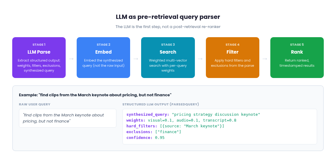
1. LLM Parse
The user's raw query goes to an LLM first. The LLM extracts a structured output containing: hard filters (metadata constraints like date ranges, speaker names, content categories), exclusions (things the user explicitly does not want), a synthesized query string that is optimized for embedding and (for multi-vector systems) dynamic modality weights for this specific query. The raw user input never gets embedded directly. The LLM produces a cleaner, more focused version.
2. Embed
The synthesized query from step 1 gets embedded with Gemini Embedding 2. Because the LLM has already stripped out negations, filters and noise, the resulting embedding is a better representation of what the user actually wants to find.
3. Search
For fused embeddings, this is a single index lookup using the clean embedding. For multi-vector retrieval, the embedding fans out across modality indices with the per-query weights from step 1 applied to score fusion. A transcription-heavy query like "what did she say about revenue growth" gets weights skewed toward the transcription index. A visual query like "the play where the defender slides" gets weights skewed toward visual.
4. Filter and exclude
The search results are filtered by the hard constraints and exclusions from step 1. Results that match excluded terms or fall outside the metadata filters are removed before the user ever sees them.
5. Rank and return
The remaining results are ranked by their (weighted) fusion scores and returned to the user.
This architecture means the LLM adds latency only once, at the very start and that cost is fixed regardless of corpus size or which embedding approach you chose. Everything downstream (embedding, search, filtering) operates on clean, structured inputs and runs at the same speed it always did.
Why the LLM belongs before search, not after
The critical problem with post-retrieval re-ranking is that it can only work with what the vector search already found. If the initial retrieval missed the best results because the raw query embedded poorly, no amount of re-ranking fixes that. Garbage in, garbage out.
Consider a query like "show me clips from the product launch but not the ones about pricing." If you embed this query as-is, the embedding will actually be closer to clips about pricing, because "pricing" is a prominent semantic signal in the query text. Vector spaces do not understand negation. The word "not" does not reverse the direction of an embedding. Your retrieval will actively return the wrong results and a post-retrieval re-ranker would then have to fix mistakes that should not have happened in the first place.
With an LLM query parser, the negation is handled before embedding. The LLM extracts "pricing" as an exclusion and produces a synthesized query like "product launch demo clips" for embedding. The embedding now points in the right direction and the exclusion filter removes pricing-related results after search. The system finds what the user wanted on the first pass.
The synthesized query does more than just strip negations. The LLM can enrich and expand the query to improve embedding quality. A user who types "frontend developer" might get a synthesized query like "frontend web developer software engineering JavaScript React TypeScript." The LLM understands the implicit context and expands the query with related terms that the embedding model can use to find better matches. The raw query is terse and ambiguous. The synthesized query is dense with semantic signal. This enrichment happens before embedding, so the vector search operates on a much better representation of intent than the user's original input would produce.
Structured outputs for reliable parsing
The practical key to making this work is structured outputs. Rather than asking the LLM for free-form text, you constrain the output to a defined schema. Using Pydantic (for Python) or equivalent schema definitions, you define the exact shape of what the LLM returns:
from pydantic import BaseModel, Field, model_validator

class ModalityWeights(BaseModel):
    visual: float = Field(default=0.33, ge=0.0, le=1.0)
    audio: float = Field(default=0.33, ge=0.0, le=1.0)
    transcription: float = Field(default=0.34, ge=0.0, le=1.0)

    @model_validator(mode='after')
    def normalize_weights(self):
        total = self.visual + self.audio + self.transcription
        if total > 0:
            self.visual /= total
            self.audio /= total
            self.transcription /= total
        return self

class HardFilter(BaseModel):
    field: str          # e.g., "date", "speaker", "content_type"
    operator: str       # e.g., "equals", "gte", "contains"
    value: str          # e.g., "2025-Q4", "CEO", "keynote"

class ParsedQuery(BaseModel):
    synthesized_query: str = Field(
        description="Cleaned, embedding-optimized version of the user's intent. "
                    "Strip negations, filters and noise."
    )
    weights: ModalityWeights = Field(default_factory=ModalityWeights)
    hard_filters: list[HardFilter] = Field(default_factory=list)
    exclusions: list[str] = Field(
        default_factory=list,
        description="Terms or concepts the user explicitly does NOT want."
    )
    confidence: float = Field(
        default=1.0, ge=0.0, le=1.0,
        description="How well the LLM understood the query intent."
    )
A query like "find clips from the March keynote where someone discusses pricing, but not the finance section" would produce a ParsedQuery with synthesized_query set to "discusses pricing in keynote presentation," weights skewed toward transcription (e.g., 0.1 visual, 0.1 audio, 0.8 transcription), a hard_filter constraining content source to the March keynote and "finance" in the exclusions list.
The default values in the schema are important. If the LLM cannot confidently determine modality weights, it returns equal defaults and the system falls back to baseline behavior. The confidence field lets you implement fallback logic: under a certain threshold, you might skip the LLM's weight suggestions and use your fixed or anchor-based weights instead.
Structured output support is now available across major LLM APIs (Gemini, Claude, etc.) and it eliminates the parsing fragility that made earlier LLM-in-the-loop approaches unreliable. To use it, pass the ParsedQuery schema as the response_format parameter (or equivalent, depending on your SDK) in your LLM API call and the model will return a JSON object conforming to the schema. You get deterministic output shapes that slot directly into your pipeline logic.
Handling negation and hard filters
Negation is the most compelling reason to put an LLM at the front of the pipeline. Vector spaces do not have a concept of "not." The embeddings for "a dog" and "not a dog" are nearly identical, not opposite. Without pre-retrieval parsing, your only option is to hope the raw query embedding somehow avoids matching negated concepts, which it will not.
With the LLM parser, negation becomes explicit. The query "find clips about the product but not finance" gets decomposed into a synthesized query ("product clips") and an exclusion list (["finance"]). The exclusion is applied as a filter after search, removing any results whose metadata or content matches the excluded terms. This is reliable and deterministic, not probabilistic.
Hard filters work the same way. "Find clips from the March keynote where someone mentions pricing" becomes a synthesized query ("mentions pricing") with a hard filter on content source ("March keynote"). The hard filter is applied at the database level during or after search, which is both faster and more reliable than trying to encode a metadata constraint into an embedding.
The LLM can also handle progressive filter relaxation. If the initial search with all filters applied returns too few results, the system can selectively relax constraints and re-query. The key is to define a priority ordering for which filters drop first. Temporal constraints (date ranges, recency) and soft preferences are typically the first to relax. Content source filters and core topic constraints are stickier. Exclusions (things the user explicitly said "not") should almost never be relaxed, since dropping an exclusion means returning exactly what the user asked to avoid. Defining this priority hierarchy upfront, either in the Pydantic schema itself (with a priority field on each filter) or as application-level logic, makes relaxation deterministic rather than ad hoc.
UI/UX considerations
Putting an LLM at the front of the retrieval pipeline has implications for the user experience that go beyond retrieval quality.
Latency expectations shift
Adding an LLM parsing step introduces latency before results begin loading. The LLM call typically takes hundreds of milliseconds, sometimes more depending on the model and query complexity. The common mitigation is to show a brief "understanding your query" indicator while the parse runs, then load results normally once the structured output is available. Because the LLM call happens once per query (not once per result), the latency is bounded and predictable.
Explainability becomes a feature
Because the LLM parse produces structured, human-readable output (the synthesized query, the weights, the filters, the exclusions), you can surface that information in the interface. A search result page that says "Searching for: 'product launch demo clips' | Weighted toward: visual (0.7) | Excluding: pricing content | Filtered to: March 2026" gives users transparency into what the system understood. This is especially valuable in enterprise contexts where users need to trust search results and want to know why certain results appear or do not appear.
Natural language query refinement
Once you have an LLM parsing layer, you can support multi-turn conversational refinement. A user searches for "product demo clips," sees results, then says "actually only the ones where they show the mobile app." The LLM parser processes this as a refinement of the previous query, adding "mobile app" to the filters or adjusting the synthesized query. The previous search context carries forward and only the delta changes. This makes the search experience feel like a conversation rather than a keyword box.
The cost question
Every LLM parse call costs tokens. But because you are parsing the query (short input, structured output) rather than re-ranking dozens of results with full context, the per-query cost is small. This scales well even at high query volumes, especially with smaller, faster models that are sufficient for query decomposition tasks. One optimization worth noting: structured extraction tasks like query parsing do not require full chain-of-thought reasoning. Most LLM APIs now expose a reasoning effort or thinking budget parameter. Disabling extended reasoning for your query parser can cut latency by 5 to 6x and cost by a similar factor with no measurable quality loss on extraction tasks. You are asking the model to fill in a schema, not to reason through a complex problem. Save the reasoning budget for tasks that actually need it.
Where LLM parsing fits in the stack
The LLM query parser does not replace the embedding and weighting strategies we covered earlier. Rather, it is the orchestration layer that makes them work together intelligently. Whether you are running a single fused index or three separate modality indices, the parser sits in front and ensures that what enters the retrieval pipeline is clean, structured and intent-aware.
For fused embedding systems, the parser provides hard filters, exclusions and a synthesized query. That alone is a significant upgrade over embedding raw user input. For multi-vector systems, the parser additionally provides dynamic weights, solving the per-query weight problem without requiring a trained ML model. In both cases, the downstream pipeline (embedding, search, filtering) operates on structured instructions rather than raw text.
The most pragmatic architecture layers these components: LLM parsing for query understanding (extract filters, exclusions, synthesized query and optionally weights), vector search for recall (find candidates using the clean embedding), score-based fusion for initial ranking (with dynamic or fixed weights depending on your architecture) and post-search filtering for hard constraints and exclusions. Each layer has a clear responsibility and you can evolve any layer independently. You can swap the LLM, change the fusion strategy, or add new filter types without re-architecting the pipeline.
Choosing the right approach
Here is a quick reference for mapping your situation to a starting architecture:
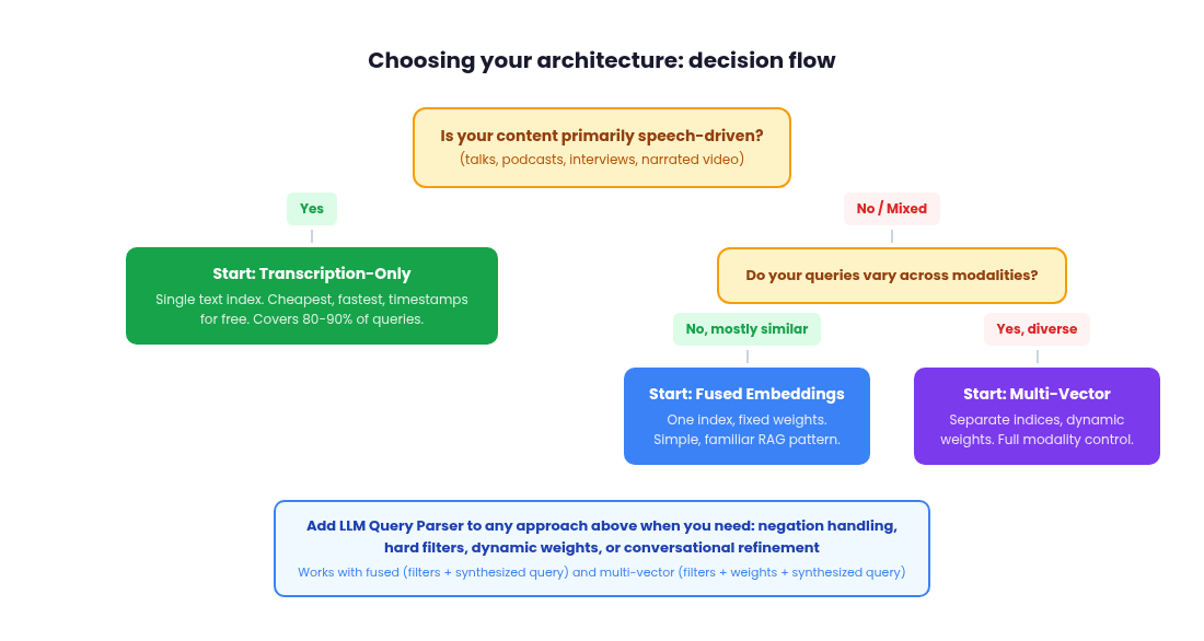
The choice between fused and multi-vector retrieval is about how much modality-level control you need. The choice to add an LLM query parser is orthogonal: it improves either architecture by providing cleaner embeddings, structured filtering and exclusion handling. For multi-vector systems, it additionally solves the dynamic weight problem.
| Scenario | Recommended starting point | Add LLM parser? | Relative indexing cost |
|---|---|---|---|
| Speech-dominant content (talks, podcasts, interviews), queries target what is said | Transcription-only, single index | Yes, for filters and exclusions | Low |
| Small team, limited ML experience | Transcription-only or fused | Yes (no ML training needed) | Low |
| Mixed content, homogeneous query patterns | Fused embeddings with fixed weights | Yes, for synthesized queries | Medium |
| Visual-dominant content (surveillance, sports, product demos), queries target what is shown | Fused or multi-vector with visual-heavy weights | Optional for version 1, valuable at scale | Medium to High |
| Mixed content, diverse query patterns across modalities | Multi-vector with anchor-based or LLM-driven dynamic weights | Yes, with dynamic weights | High |
| Large team, precision-critical, willing to invest | Multi-vector with full LLM pipeline | Yes, with eval-driven weight tuning | High |
| Users need negation, hard filters, conversational refinement | Any embedding approach | Required | Depends on approach |
For most teams, the practical decision comes down to two questions:
1. How diverse is your query distribution?
If most queries favor similar modality balances, static approaches (fused or fixed-weight multi-vector) are likely sufficient. If query intent varies significantly across modalities, multi-vector retrieval with LLM-driven dynamic weights becomes the higher-ROI investment. If your users regularly use negation, hard filters, or compositional logic, an LLM query parser pays for itself regardless of which embedding approach you chose.
2. What expertise and operational capacity does your team have?
Fused embeddings require minimal specialized skill. Fixed-weight optimization requires data science capability. Anchor-based routing requires thoughtful design but avoids ML training overhead. LLM query parsing requires prompt engineering and structured output design but no custom model training and it delivers the broadest capability uplift for the effort involved.
These approaches are not mutually exclusive. In fact, the best production systems layer them. Even a fused embedding system benefits from an LLM parser that extracts filters and exclusions before embedding. A multi-vector system gets the additional benefit of per-query dynamic weights. Start simple, gather real query data and user feedback and evolve incrementally. A working system with fixed weights will teach you more about your query distribution in one month of production traffic than six months of theoretical planning.
The key is to design for incremental upgrades from the start. If you begin with multi-vector retrieval and separate indices, every subsequent improvement (dynamic routing, LLM query parsing, conversational refinement) is an additive change, not a re-architecture. The indexing work you do today carries forward as your retrieval sophistication grows. And with models like Gemini Embedding 2 making multimodal embeddings accessible through a single API call, the barrier is no longer the model. It is the system design around it.
Evaluating retrieval quality
None of the architectural decisions matter if you cannot measure whether your system is actually returning good results. Evaluation is what turns intuition into evidence and it does not need to be complicated to be useful. As covered at the start of this article, your evaluation set is the foundation of every architectural decision. This section covers how to construct it in detail and how to use it once your system is in production.
Build a golden evaluation set
Start by collecting 50 to 100 real user queries paired with the correct result (or results) each query should return. These do not need to be exhaustive. Even a small set of hand-labeled pairs gives you a stable baseline to test against. Pull queries from actual user sessions if you have them, or write representative queries yourself based on the content types you are indexing. Each entry should include the query text, the expected video or segment ID and ideally the expected timestamp range for segment-level retrieval.
The key discipline is labeling per-modality. For a query like "find the moment the speaker mentions churn rate," the correct result is a transcription match. For "show me the chart comparing Q3 and Q4," it is a visual match. Tag each eval pair with which modality should be the primary signal. This lets you evaluate each retrieval path independently rather than only measuring the blended output.
Metrics that matter
For most production systems, two metrics give you 80% of the signal you need.
Precision@k
Of the top K results returned, what fraction are relevant? If 8 of 10 returned video segments actually match the query intent, precision@10 is 0.80. Use this when users only look at the top few results.
Recall@K
Of all relevant segments in the dataset, what fraction did you find in the top K? This is harder to measure because you need to know the total set of relevant items, which is rarely possible at full corpus scale. Most teams approximate recall using their golden evaluation set rather than the full corpus.
Mean Reciprocal Rank (MRR)
Tells you how high the first correct result appears. An MRR of 1.0 means the right answer is always first. An MRR of 0.5 means on average, the right answer is second.
NDCG (Normalized Discounted Cumulative Gain)
Are the best results ranked highest? Surfacing the perfect moment at position 1 counts more than at position 10. NDCG penalizes good results buried low in the ranking, but it requires graded relevance labels (e.g., perfect match = 3, partial match = 1, irrelevant = 0) to be most useful.
Filter accuracy
For LLM query parser pipelines specifically, when the user asks for "clips from the March keynote," does the system return only segments from that keynote? Binary pass/fail per filter.
Filter extraction rate
Did the LLM correctly extract all implied filters from the natural language query? This isolates parser failures from embedding failures.
Latency
Time per query, measured end to end including LLM parsing, embedding, search, filtering and ranking.
Cost per query
Tokens consumed and dollars spent per query, useful for projecting costs at production scale.
Failure mode tagging
When a query fails, categorize why. Wrong modality weighted? Missed exact phrase? Exclusion not applied? This is less a metric and more an evaluation discipline, but it is what turns metrics into prioritized fixes.
Track these per-modality, not just in aggregate. If your transcription retrieval has an MRR of 0.9 but your visual retrieval is at 0.4, that tells you exactly where to invest. It might be a weight calibration issue, a score threshold problem, or a sign that your visual embeddings need better preprocessing (e.g., extracting keyframes rather than embedding raw video segments).
Pick the metrics that match how your users will interact with results. If they only look at the top three, optimize for precision@3. If they scan a longer list, NDCG matters more. If your use case requires negation and filtering, track filter accuracy alongside retrieval quality.
Once you have an evaluation set and a metric, every architecture question becomes empirical
Should you use fused embeddings or multi-vector retrieval? Run both against your evaluation set and compare. What modality weights work best? Sweep through combinations and measure. Is transcription-first sufficient, or do you need visual embeddings? Test transcription-only first, see where it fails and add modalities based on actual failure cases rather than assumptions.
Working backward from evaluation forces you to be honest about what your system needs to do. Without it, you are guessing. With it, every decision in the rest of this article becomes a measurable trade-off rather than a judgment call
Weight tuning with evaluation data
Once you have an eval set, optimizing fusion weights becomes empirical rather than guesswork. For fused embeddings, sweep through weight combinations at reasonable granularity (e.g., increments of 0.05 across your three modalities) and measure precision@k on your eval set for each combination. For multi-vector systems, do the same sweep on your fixed baseline weights and separately evaluate whether LLM-driven dynamic weights outperform the best fixed configuration across your eval set.
This is also where you validate score thresholds. Run your eval queries, collect the similarity scores for both relevant and irrelevant results and plot the distributions. The right threshold is the one that maximizes the gap between the two distributions for each modality. If the distributions overlap heavily for a particular modality, that is a signal that the modality is not discriminating well for your content type and you may want to down-weight it.
Monitoring in production
Eval sets tell you how the system performs at a point in time. Production monitoring tells you when things drift. Track the distribution of similarity scores over time, both the mean and the spread. If your average top-1 score starts dropping, it could mean your content library has grown into domains your embeddings handle poorly, or that user query patterns have shifted away from what your weights are tuned for.
Log a sample of low-confidence results (where the top score barely clears your threshold) and periodically review them manually. These edge cases are where your system is most fragile and they are the best source of new eval pairs. A lightweight feedback loop (even just a thumbs-up/thumbs-down on search results in your UI) compounds over time into a high-quality eval dataset that reflects real usage patterns rather than synthetic assumptions.
Need help building advanced retrieval systems?
Easie helps teams design and ship multimodal search, RAG pipelines and AI-powered retrieval infrastructure. If you are working through the decisions in this article and want hands-on guidance, please reach out.